Logistic Regression Explained: The Math & Code Behind Classification

Logistic regression is widely used for binary classification. This post explains its probability-based foundation, derives the gradient ascent, and shows how to implements all this in Python.

Logistic Regression Explained

Logistic regression is an ML method used to classify data into two categories. It’s called “logistic” because it uses the logistic function to model the probability of a binary outcome. Logistic regression tries to minimize the empirical risk.

Once we have the optimal weights, we can easily predict the class of a new data point:

Mathematically, logistic function is

Using this in logistic regression we get

What this means. is that the probability of a data point being in class 1 ig given by that logistic function. Because we use logistic function for binary data (0 or 1), we can also predict the data point being in class 0:

And if we have N data points, each with feature vector $x_n$ and label $y_n$ , we can write the likelihood functions as:

and

Bernoulli Distribution

Before we can write the likelihood function, we must understand the Bernoulli distribution. The Bernoulli distribution is a simple probability distribution for random variable that can take only two values.

The basic idea of it is that it “flips” value to 1 in probability $p$ and 0 in probability $1 - p$ .

In logistic regression, we have a similar goal, we want to predict the probability of the label being 1 or 0. So let’s use Bernoulli distribution to model the probability of the label being 1 or 0. First we define the probability for flipping to 1 as

This is also called as the sigmoid function. After that we can use the same logic as in the Bernoulli distribution to model the probability of the label being 1 or 0.

This works for single data point, but we want to model the probability of the label being 1 or 0 for all data points. Thus we can assume that each $y_n$ is independent of each other given the weights $\mathbf{w}$ . So we can write the likelihood function as:

This is also called as the likelihood function:

However, this is a product of probabilities, which is hard to work with. So we take the logarithm of the likelihood function to get the log-likelihood function:

which can be further simplified using logarithmic rules to:

Optimization & Learning Approach

We now have our likehood function, but we need to find the weights that maximize it. So we need to find the weights that maximize the log-likelihood function.

Well, now that we know what we want to maximize, we also need to find a way to do it. This is where gradient ascent comes in. I have written about gradient descent in my previous posts, so I won’t go into too much details. How gradient ascent differs from gradient descent is that we are trying to maximize the function, not minimize it.

So our log-likehood function becomes:

where

We need gradient of this in respect to the weights. So let’s calculate it for only single term first.

Let’s derive it in respect to the weights.

We can notice that $z_n=w^Tx_n$ , so by the chain rule we have

Then we can get the sigmoid function using the chain rule

Differentiating the first part gives us:

and the second part

Combining this result with the previous one we get:

and by factoring we finally obtain:

Inside part of the brackets can be simplified to

Thus for single point we get

Now that we know how to get the gradient for a single point, we can get the gradient for the whole dataset by summing over all points:

Unlike gradient descent (which minimizes error), we use gradient ascent because we are maximizing the likelihood function. Thus the rule for updating the weights is

Implementation

Now that we have the gradient descent rule, we can implement it in Python. We will use NumPy for matrix operations. First, let import the necessary libraries and generate some data to test our implementation:

import numpy as np
import matplotlib.pyplot as plt

np.random.seed(42)
num_samples = 200
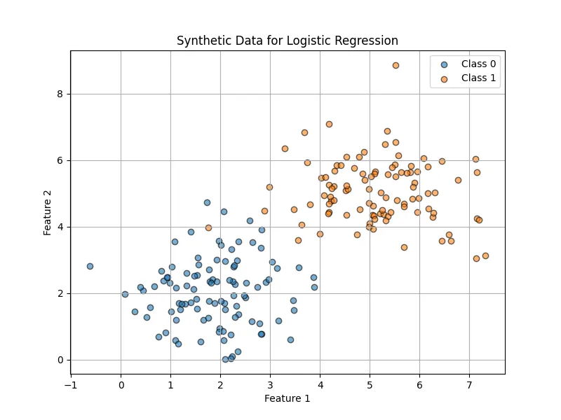
x1_class0 = np.random.normal(loc=2, scale=1, size=(num_samples // 2, 2))
x1_class1 = np.random.normal(loc=5, scale=1, size=(num_samples // 2, 2))

y_class0 = np.zeros((num_samples // 2, 1))
y_class1 = np.ones((num_samples // 2, 1))

X = np.vstack((x1_class0, x1_class1))
y = np.vstack((y_class0, y_class1)).flatten()

The data is visualized as follows:

After that I preprocess the data.

N = len(X)
train_ratio = 0.8
train_size = int(N * train_ratio)

indices = np.random.permutation(N)
train_idx, test_idx = indices[:train_size], indices[train_size:]
X_train, y_train = X[train_idx], y[train_idx]
X_test, y_test = X[test_idx], y[test_idx]

X_train = np.hstack((np.ones((X_train.shape[0], 1)), X_train))
X_test = np.hstack((np.ones((X_test.shape[0], 1)), X_test))

mean_X_train = np.mean(X_train[:, 1:], axis=0)
std_X_train = np.std(X_train[:, 1:], axis=0)

X_train[:, 1:] = (X_train[:, 1:] - mean_X_train) / std_X_train
X_test[:, 1:] = (X_test[:, 1:] - mean_X_train) / std_X_train

Notice that we add a column of ones to the data to account for the bias term in the hypothesis function. Why is that?

The bias term is a constant that allows the model to shift the decision boundary away from the origin (0,0). This way our decision boundary is not forced to pass through the origin, which makes the model more flexible and allows it to fit the data better. Also, we normalize the data to have zero mean and unit variance. This is important because it ensures that the features are on the same scale, which helps the gradient descent algorithm to converge faster.

Then we define the gradient ascent algorithm to find the optimal weights.

learning_rate = 0.01
num_iterations = 1000
weights = np.zeros(X_train.shape[1])

def sigmoid(z):
    return 1 / (1 + np.exp(-z))

for i in range(num_iterations):
    preds = sigmoid(np.dot(X_train, weights))
    gradient = np.dot((y_train - preds), X_train)
    weights += learning_rate * gradient

We notice that the weight update rule is same as the one in the math section!

Let’s see how well our model performs on the test set.

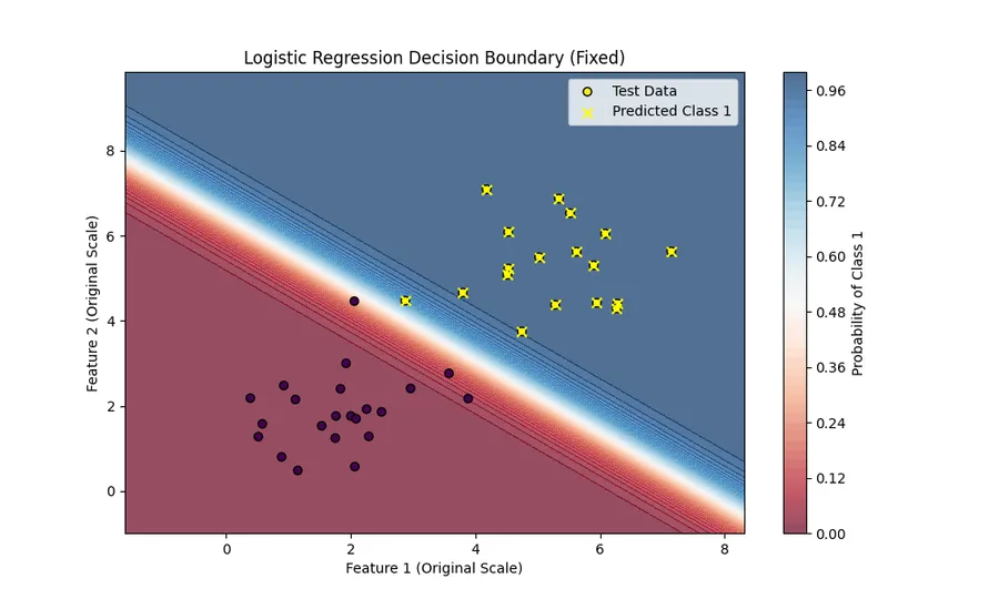
test_preds = sigmoid(np.dot(X_test, weights))
predicted_labels = (test_preds >= 0.5).astype(int)

accuracy = np.mean(predicted_labels == y_test)
print(f"Accuracy: {accuracy * 100:.2f}%")

Accuracy: 100.00% Works great! Our model has 100% accuracy on the test set.

I also visualized the decision boundary of our model to this picture.

Summary

In this post we learned the basics of logistic regression and how it can be used to classify binary data. Oour model was able to achieve 100% accuracy on the test set.

For the full code, you can check out the GitHub repository.