Shrinking Embeddings: Real Results with Mathryoshka Models

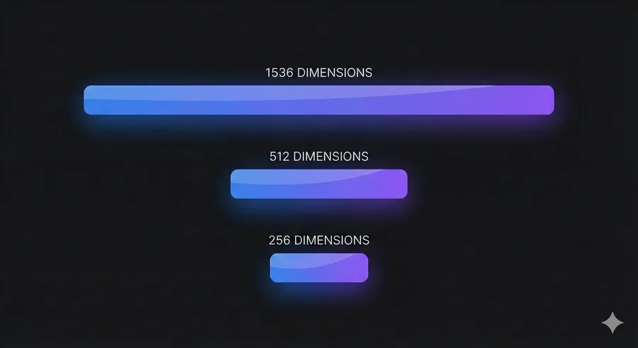
Shrinking embeddings is a big topic right now. People say you can take the prefix of these new models like OpenAI’s text-embedding-3-small, and still get almost the same performance. This comes from Matryoshka Representation Learning (MRL), a training method that should let you chop a 1536-dim vector down to something much smaller without breaking everything.

At least in theory. So I tested it on my own dataset of 10,000 attractions and real user-style queries. And yes, shrinking works, but not quite the way I expected.

In this post I’ll explain how MRL actually works and show my real results. The short version: you can shrink embeddings, but it heavily depends on your actual problem. Some dimensions carry more weight than others… just not always in the way the papers make it sound.

Learned Representations Are Not Efficient

Before jumping into MRL, it’s worth covering what we’re actually shrinking. Embedding models like text-embedding-3-small output what’s called a learned representation:

Learned Representation: How a model internally describes or encodes information after training, instead of using manually-designed features.

In practice this means the model gives us a big list of numbers. We don’t decide what each dimension means. We don’t design features. The model figures out whatever structure it needs during training.

Then we take these vectors and use them in downstream applications: anything from similarity search to clustering to RAG.

The problem is that learned representations are not necessarily efficient. Even simple tasks get a huge vector. text-embedding-3-small outputs 1536 dimensions. That’s already the “small” model.

Why This is Inefficient

If you force a model to produce only 64 dimensions, it must compress all useful information into those 64 numbers. But if it outputs 3072? It spreads information across all 3072 dimensions, even when the task doesn’t need that much capacity.

So we end up with:

1. Info is not organized efficiently

Computations always use the full vector, even if only a small part of it carries most of the signal.

2. Small and large versions need to be trained separately.

You can’t just slice off the first 128 dimensions (or take a random subset) and expect it to work. The model wasn’t trained with that constraint.

3. Storage and compute explode at scale.

This matters in real applications.

In my case:

a single embedding (3072 dims) → ~12 KB

10,000 attractions → ~117 MB just for raw vectors

And similarity search is basically a dot product across all dimensions, so doubling the vector size doubles that cost too.

4. We can’t cheaply adapt embedding size per use case

Even if your task is very easy, you still pay the cost of the full vector. And since the model didn’t learn any explicit structure in the dimensions, you can’t just “pick the first 256” and call it a day.

Mathryoshka Representations

In the previous section, I said we can’t just take a random subset of an embedding and expect it to work well. But what if the model was trained so that subsets actually do work?

Since models are trained end-to-end, we can change how dimensions behave simply by changing the loss function. This is the core idea behind Matryoshka Representation Learning (MRL): train the model so that the first N dimensions already produce a useful embedding, and additional dimensions refine it.

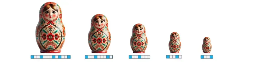
The name of the technique comes from the Russian Matryoshka dolls, where smaller dolls are nested inside larger ones. MRL does the same thing with embeddings: smaller prefixes sit “inside” the larger vector and remain meaningful on their own.

For example, if we have embedding vector of size 1024, we can take prefixes of size 512, 256, 128, 64 and expect that the first dimensions in the output are more “coarse”, e.g. their importance is higher for the final output. How is this is achieved is by clever trick, where instead of calculating loss for the whole model, we actually calculate loss as sum of all the interested loss prefixes:

$Loss_{full} = Loss_{1024} + Loss_{512} + ... + Loss_{64}$

To minimize this combined loss, the model must ensure that each prefix is individually useful. This naturally pushes the important, coarse information toward the beginning of the vector. Adding more dimensions still helps but mostly with finer distinctions.

At What Cost?

Does forcing this structure hurt the full-dimensional performance?

Surprisingly, no.

The original MRL paper shows that in full dimensionality performance of the MRL does match or even sligthly improve the standard model. Which might seem weird at first, since we are forcing the structure of dimensions be coarse-to-fine.

This sounds odd at first: we’re forcing structure into the representation, shouldn’t that limit the model? But remember, modern models are heavily overparameterized. They have more than enough capacity to give good results at every prefix and still make use of the full dimensionality.

Empirically we see that

• small prefixes already capture most of the task-relevant signal (coarse info),
• while adding dimensions consistently improves performance (finer info),
• and full-dimensional performance matches a standard model.

Slack in Representations

The power of MRL comes from the simple fact that modern embedding models are massively overparameterized. They output far more dimensions than most tasks actually need.

That means there’s a lot of slack: redundancy in the representation. Because of this extra space, the model can reorganize information (coarse → fine) without hurting the final performance.

If we had a model with no slack, meaning every dimension was already fully optimized for the task, MRL would be too strong of a constraint. Forcing every prefix to work would push the model away from the optimal solution.

But with large, overparameterized models, there’s enough room for structure to emerge, and MRL can shape the representation without sacrificing accuracy.

Implemtation

For my own experiment, I kept working on my pet-project of Chinese itineraries. I have over 10 000 attractions embedded with the text-embedding-3-small model from the OpenAI, All of the attractions are embedded by their most important information: title, description, location, rating etc.

The goal of the experiment was to see if I could reduce the dimensions of my embeddings without losing the performance on the most important task: finding the most relevant attractions based on user queries. So the first task was to generate user queries.

User Queries

What I’m interested in my application is to find the best matching attractions for user requests. So first I generated around 150 synthetic queries from the current attractions.

Generate 3 different search queries a tourist might type into a search bar to find this place:

1. A query that roughly mentions the name and city.
2. A natural language description (what it is, without exact name).
3. A "vibe" query that includes the city and the kind of experience (e.g. romantic night view, ancient temple, kid-friendly park, etc).

That type of prompt was used to generate list of queries, for example, here’s example of one:

{
  "id": "q_48_vibe",
  "text": "historic classical gardens in Suzhou tour",
  "type": "vibe",
  "attraction_id": "67e418b999321d34a70d6482",
  "location": "Jiangsu Province, Suzhou City, Gusu District"
}

Experiment

The main experiment is quite a simple after I had all the data. The basic idea was to embed the query with the same text-embedding-3-small model, and check the important metrics for all of the prefixes. I used these dimensions for testing purposes.

DIMS_TO_TEST = [64, 128, 256, 512, 1024];

and for each of the dims, I could just manually calculate the cosine similarity in the code, and use that to calculate the similarity.

for dim in dims_to_test:
  # Prefix baseline
  q_vec_d = q_vec_full[:dim]
  docs_d = doc_embeddings[:, :dim]

  start = time.perf_counter()
  scores_d = cosine_similarity_matrix(q_vec_d, docs_d)
  latency_ms = (time.perf_counter() - start) * 1000.0

  rho = spearman_from_scores(scores_full, scores_d, TOP_N_FOR_SPEARMAN)
  overlap = overlap_at_k(scores_full, scores_d, OVERLAP_K)
  # Outputs

Important thing in my experiment was that I tested how well the model did with using the first N amount of dimensions for the task versus using random subset of size N dimensions to the task to see if there really is Mathryoshka behaviour in the embeddings.

Results

The results for the task were quite interesting. The latency graph had no suprise:

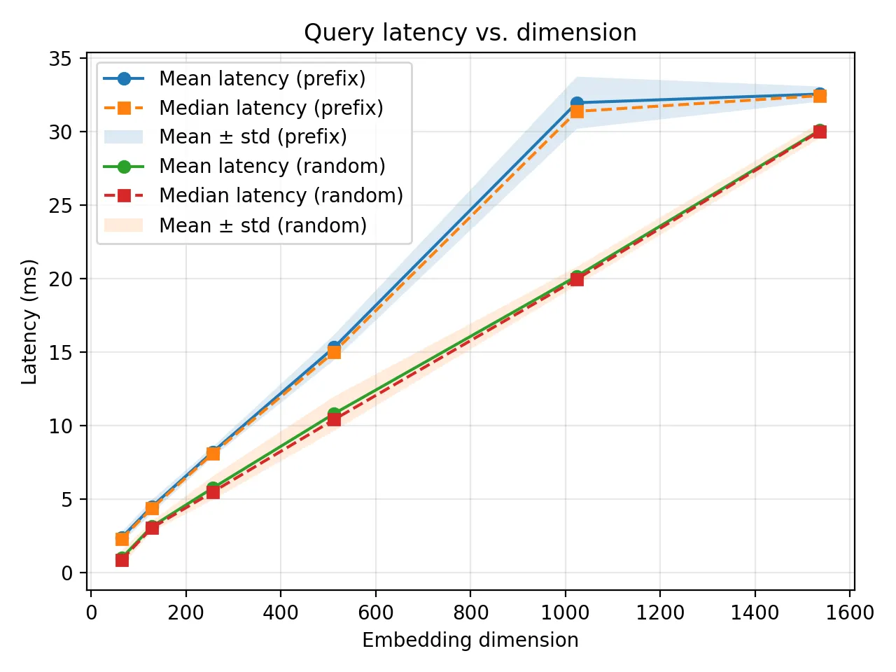
The latency of the prefix is all the time better, due to memory access being contiguous.

The rest of the metrics, though, were surprising. Not because they were bad, but because the difference between the prefix and a random subset was much smaller than I expected.

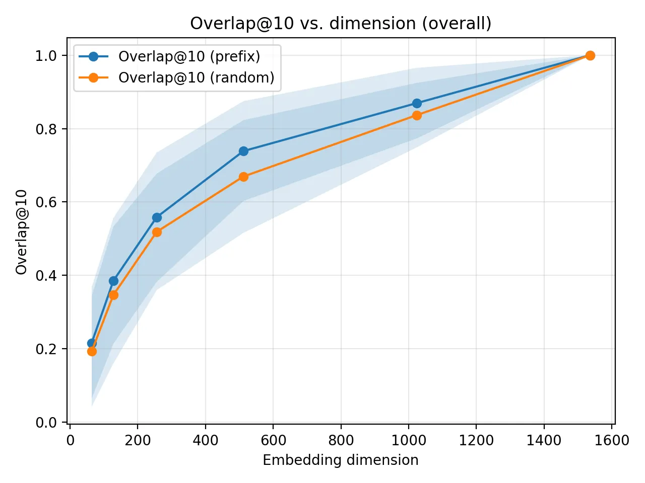
I tested Overlap@10, which measures how many of the top-10 results match the full-dimension model. Here, the random subset baseline performed far better than I thought it would.

MRL still beats the random subset at every dimension, so the first dimensions do contain more useful information, but the margin is subtle.

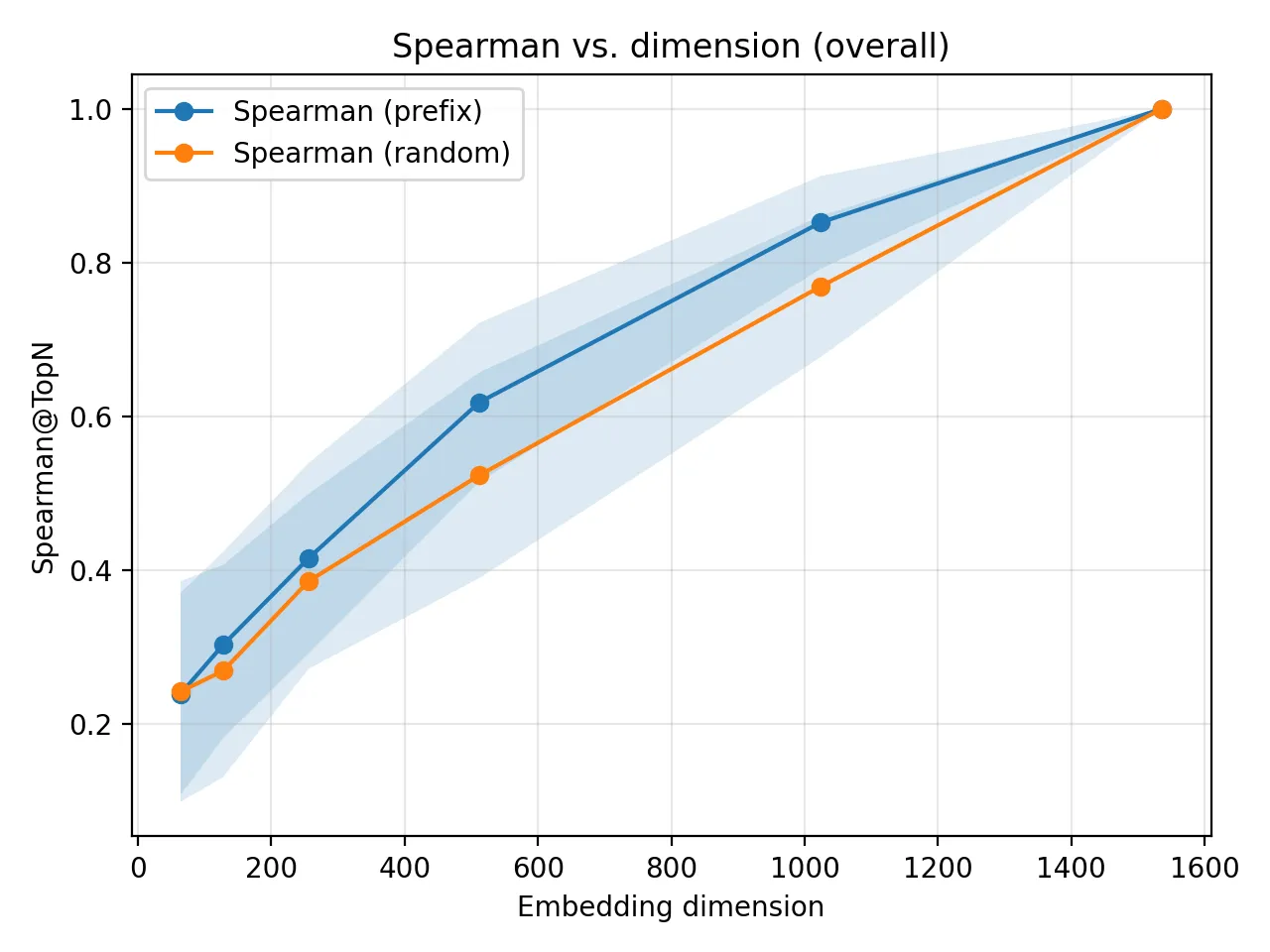
Spearman rank correlation was the most underwhelming metric. But in hindsight, this makes sense: Spearman is extremely sensitive to even tiny changes in ranking, and my dataset contains many attractions that are semantically similar. Small movements in rank → big drop in Spearman. So this metric exaggerates differences that don’t matter for retrieval.

The metric that actually matters for my application is Recall@10: whether the correct attraction appears anywhere in the top 10.

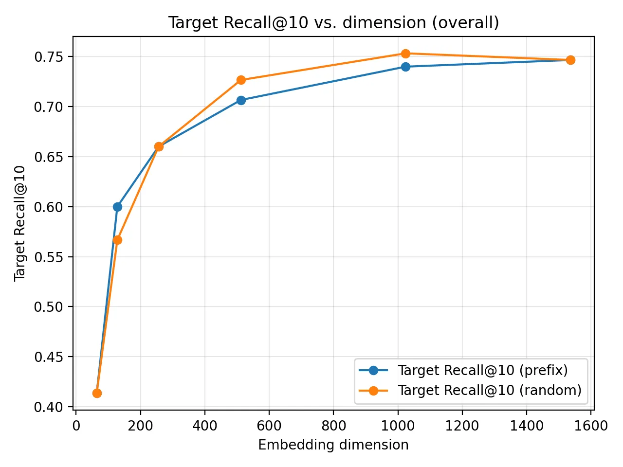
And this was the biggest surprise. The random subset almost matched the prefix, and in a few dimensions it was even slightly better. Since MRL-trained embeddings are supposed to push the “important” information to the start of the vector, I expected the random slice to fall apart. Instead, it held up extremely well.

The explanation is pretty simple: my attractions cluster semantically, the model is heavily overparameterized, and Recall@10 doesn’t care about exact ranking within the top 10. So as long as the random slice keeps enough coarse information to land the correct attraction somewhere in the top 10, it performs fine.

Conclusion

So what can I conclude from the experiment? The most important thing is how can I use the information I gathered, and as we can see from the recall of top 10 attractions, it is almost as strong as the full vector in 512 dimensions!

The performance dropped from 0.74 to 0.71 by reducing the size of the dimensions by 3x! This is huge for the speedup of my application, and the storage. I get 3x smaller embeddings and 2-3x speedup for the pure-vector calculations, by losing almost no performance.

Learnings

In this blog I went over Matryoshka Representation Learning and applied it to my own use case. Modern embedding models already use this technique, and it really does let us shrink vectors without losing much performance.

But MRL isn’t magic. In my experiment it worked, the prefix slices were consistently better, but the difference was smaller than I expected. The random subsets were surprisingly strong and, in some metrics, almost matched the prefixes. So yes, text-embedding-3-small clearly has some Matryoshka structure, but that doesn’t automatically translate to dramatic gains in every task.

The bigger lesson is this: learned representations are heavily overparameterized, and that’s actually an advantage. Because of this slack, we can safely shrink embeddings and still keep almost all of the practical performance, while getting huge wins in compute and storage.

And for my use case, going from dimensions of 1536 to 512 means almost no loss in Recall@10, while getting 3x smaller vectors and 2-3x speedup in similarity search. That alone makes it worth it.